Transfer learning with VGG16 and VGG19, the simpler way!

What is Transfer learning?
In transfer learning, we use an existing model to solve different but related problems. Basically, we try to exploit what has been learned in one task and improve generalization in another task. We use the model’s pre-trained weights or model architecture to solve our problem. In this blog, we are using the pre-trained weights of VGG16 and VGG19, change the output layer and solve a classification problem on the flower dataset.
Is transfer learning advantageous?
Yes, it is! Transfer learning saves training time, gives better performance in most cases, and reduces the need for a huge dataset. It isn’t a generalized method but helps in solving related problems.
Any existing Transfer learning methods to start with?
Keras applications have given users access to architectures such as VGG16, VGG19, RESNET, and a lot more. There are 25+ models available, with mention of their top accuracies on ImageNet classifications, parameters, depth, and size. You can access the models here. Let’s explore two models, know-how these architectures are!
VGG-16
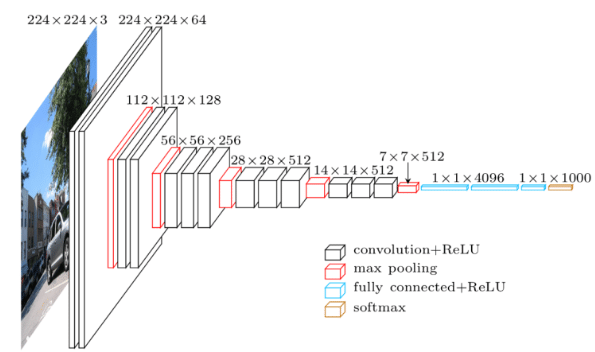
Published in 2014, VGG16 [Visual Geometry Group — 16] is one of the simplest CNN architectures used in ImageNet competitions. Taking out the ambiguity of filter size, kernel size and padding, VGG16 is structured as follows:
All convolution layers in VGG-16 have
- Filter size — 3x3
- Stride — 1
- Padding — Same
All Max-pooling layers in VGG-16 have
- Filter size — 2x2
- Stride — 2
2Conv — 1Maxpool — 2Conv — 1Maxpool — 3Conv — 1Maxpool — 3Conv — 1Maxpool — 3Conv — 1Maxpool — 1FC — 1FC — 1FC

The architecture has 13 convolutional layers followed by 3 fully connected layers, adding up to 16 layers to learn weights and bias parameters and hence the name VGG-16.
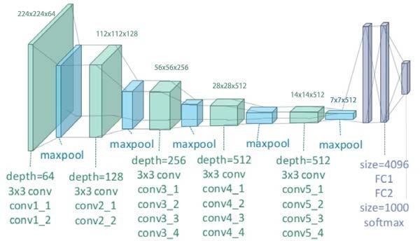
VGG-19
VGG-19 architecture is very much similar to VGG-16. We have 3 additional convolutional layers for the VGG-16 network. The architecture is as follows:
2Conv — 1Maxpool — 2Conv — 1Maxpool — 4Conv — 1Maxpool — 4Conv — 1Maxpool — 4Conv — 1Maxpool — 1FC — 1FC — 1FC

VGG-16 and VGG-19 architectures, due to their depth are slow to train and produce models of very large size. Though the architectures we see here are different, we can create a simple template to perform transfer learning from these models with few lines of code. The following snippet of code can help in performing the required classification task.
Transfer learning template
#import required libraries — we do need the models, flatten, dense, input layers
import numpy as np
import pandas as pd
from glob import glob
import matplotlib.pyplot as plt
from tensorflow.keras.layers import Input, Lambda, Dense, Flatten
from tensorflow.keras.models import Model
from tensorflow.keras.applications.vgg16 import VGG16
from tensorflow.keras.applications.vgg19 import VGG19
from tensorflow.keras.preprocessing import image
from tensorflow.keras.preprocessing.image import ImageDataGenerator
from tensorflow.keras.models import Sequential
Once the required libraries are imported, pre-process the inputs. The dataset we have is on flower recognition with 4242 images of flowers, categorized into 5 classes.
# Path for train, validation and test datasets
train_path = 'Datasets/train'
valid_path = 'Datasets/test'
test_path = 'Datasets/val'IMAGE_SIZE = [224, 224] #Default image size for VGG16folders = glob('Datasets/train/*') #Get number of classes# ImageDataGenerator can help perform augumentation on existing images. This way, we get more diverse train set.
train_datagen = ImageDataGenerator(rescale = 1./255, shear_range = 0.2, zoom_range = 0.2, horizontal_flip = True)
validation_datagen = ImageDataGenerator(rescale = 1./255)
test_datagen = ImageDataGenerator(rescale = 1./255)#Through flow_from_directory - we create an array of images that can be used for training.
training_set = train_datagen.flow_from_directory(
'Datasets/train',
                                                 target_size = (224, 224),
                                                 batch_size = 64,
                                                 class_mode = 'categorical')validation_set = validation_datagen.flow_from_directory('Datasets/val',
                                                 target_size = (224, 224),
                                                 batch_size = 64,
                                                 class_mode = 'categorical')test_set = test_datagen.flow_from_directory('Datasets/test',
                                            target_size = (224, 224),
                                            batch_size = 32,
                                            class_mode = 'categorical')
Please note that the image size for the VGG-16 and VGG-19 networks is 244x244. While taking any other model, please check the image size in the pre-processing stage.
# Create a VGG16 model, and removing the last layer that is classifying 1000 images. This will be replaced with images classes we have.
vgg = VGG16(input_shape=IMAGE_SIZE + [3], weights='imagenet', include_top=False) #Training with Imagenet weights# Use this line for VGG19 network. Create a VGG19 model, and removing the last layer that is classifying 1000 images. This will be replaced with images classes we have.
#vgg = VGG19(input_shape=IMAGE_SIZE + [3], weights='imagenet', include_top=False)# This sets the base that the layers are not trainable. If we'd want to train the layers with custom data, these two lines can be ommitted.
for layer in vgg.layers:
  layer.trainable = Falsex = Flatten()(vgg.output) #Output obtained on vgg16 is now flattened.
prediction = Dense(len(folders), activation='softmax')(x) # We have 5 classes, and so, the prediction is being done on len(folders) - 5 classes#Creating model object
model = Model(inputs=vgg.input, outputs=prediction)model.summary()
This gives the model that we’ve imported and change in the output layer.
#Compile the model
model.compile(loss='categorical_crossentropy', optimizer='adam', metrics=['accuracy'])
history = model.fit(training_set, validation_data=validation_set, epochs=20, batch_size=32)
The model is trained for specified epochs, and the accuracy of 82% on validation data is good for a start. Plotting the accuracy and loss for VGG16 on our dataset, we have
# loss
 plt.plot(history.history['loss'], label='train loss')
 plt.plot(history.history['val_loss'], label='val loss')
 plt.legend()
 plt.show()

 # accuracies
 plt.plot(history.history['accuracy'], label='train acc')
 plt.plot(history.history['val_accuracy'], label='val acc')
 plt.legend()
 plt.show()
If the model reaches the desired accuracy on required changes — save the model.
from tensorflow.keras.models import load_model
model.save('FlowerClassification.h5')
You can access the code on GitHub. In the upcoming article, lets explore GoogLeNet and ResNet.
